Computational Fluid Dynamics (CFD) is an important field. It stands somewhere at the crossroad of Engineering, Physics and Computer Science. Understanding CFD requires experience and opens a lot of possibilities since it has many applications, from Environmental Engineering to Aerospace and Biosciences. In this article we provide a summary of OpenFOAM from available open-source content and describe some of the basics an administrator might want to know.
Open Field Operation and Manipulation (OpenFOAM) is free software, written in C++, to analyze various CFD problems. A large number of contributors come from academia and related industries. The code is modular and open which allows users to customize and adapt it to fit the requirements of the problem that is being studied.
Over the years the codebase diverged in two different versions with different considerations and brilliant maintainers. One, hosted on GitHub, is maintained by the OpenFOAM foundation and is versioned OpenFOAM-XX. The other, hosted on GitLab, is versioned OpenFOAM-XXXX. We will not dive further into this history but rather focus on the COPR packages that are already available in Fedora Linux distributions. The libraries have a common codebase. For an introduction to OpenFOAM any version is great. As long as you understand this difference you will be able to navigate the available online documentation.
1. OpenFOAM Installation
We are installing, as of now OpenFOAM-2312, on Fedora Workstation 40 (3cpu, 4g) provisioned with Virtual Machine Manager. The following command snippets apply to these versions only.
user@fedora:~$ sudo dnf copr enable -y openfoam/openfoam
user@fedora:~$ sudo dnf install -y openfoam-default paraview setools-consoleuser@fedora:~$ rpm -ql openfoam
/usr/lib/openfoam/openfoamuser@fedora:~$ ls -la /usr/lib/openfoam/openfoam/
drwxr-xr-x. 1 root root 58 Feb 7 21:36 applications
drwxr-xr-x. 1 root root 796 Feb 7 21:35 bin
drwxr-xr-x. 1 root root 224 Feb 7 21:35 etc
drwxr-xr-x. 1 root root 1170 Feb 7 21:36 src
drwxr-xr-x. 1 root root 462 Feb 7 21:35 tutorials
The default installation bundle contains the compiled binaries, the docs and the tutorials folder. The source code for the main solvers and tools, used throughout the tutorials, are found in the applications folder. The src folder contains the main cpp core libraries.
Notice the permissions are rwxr-xr-x (755), so we should be able to read/execute openfoam as a rootless user.
/usr/bin/openfoam is not a binary but a shell script that passes any arguments down the call to a Bash interactive script. This script loads a session with a set of environment variables and other prerequisites like Lua modules etc. Let’s create a rootless user (“ofuser”) with openfoam as its default shell. This is the user we will use henceforth.
user@fedora:~$ sudo useradd --create-home --shell /usr/bin/openfoam
--selinux-user user_u ofuser --groups systemd-journal
user@fedora:~$ sudo passwd ofuser
Now login as ofuser via GNOME and open a terminal
openfoam = /usr/lib/openfoam/openfoam2312
* Using: OpenFOAM-2312 (2312) - visit www.openfoam.com
* Build: _c39a0f64-20231220
* Arch: label=32;scalar=64
* Platform: linux64GccDPInt32Opt (mpi=sys-openmpi)
OpenFOAM shell session - use 'exit' to quitopenfoam2312:~/
ofuser$ foamInstallationTest
We notice the shell changed. Now check some well known OpenFOAM environment variables that appear for this session and the Lmod status.
[ofuser$] env | grep -E "^FOAM|^WM"
FOAM_RUN=/home/ofuser/OpenFOAM/ofuser-2312/run
FOAM_TUTORIALS=/usr/lib/openfoam/openfoam2312/tutorials
FOAM_LIBBIN=/usr/lib/openfoam/openfoam2312/platforms
FOAM_APP=/usr/lib/openfoam/openfoam2312/applications
WM_PROJECT_USER_DIR=/home/ofuser/OpenFOAM/ofuser-2312
WM_PROJECT_DIR=/usr/lib/openfoam/openfoam2312
...
[ofuser$] module load mpi
[ofuser$] module list
Currently Loaded Modules:
1) mpi/openmpi-x86_64
$FOAM_LIBBIN is an important folder that contains linked shared libraries. Notice that $FOAM_TUTORIALS is part of the openfoam-default installation bundle. However, $FOAM_RUN doesn’t exist. Create $FOAM_RUN manually as follows:
[ofuser$] mkdir --parents $FOAM_RUN
[ofuser$] cp -r $FOAM_TUTORIALS $FOAM_RUN
[ofuser$] cd $FOAM_RUN/tutorials
We can test MPI (Message Passing Interface) by running the following process on three different CPUs
[ofuser$] mpiexec -np 3 taskset -c 0,1,2 sh -c 'ps -o pid,psr,comm $$'
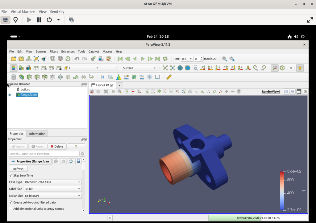
For post-processing you will use paraview or in most cases you will use the paraFoam wrapper. Once the UI opens, make sure you apply the changes, then from the top drop-down menus select the T (Temperature). You can also play the animation showcasing heat distribution over time. This model is a 3D flange file in ANSYS format that is converted into OpenFOAM format. We then simulate the distribution of temperature in time. You can see one end of the flange is heating more and more.
[ofuser$] cd $FOAM_RUN/tutorials/basic/laplacianFoam/flange/
[ofuser$] ./Allclean && ./Allrun
[ofuser$] LIBGL_ALWAYS_SOFTWARE=true paraFoam

Paraview is powerful software in itself, independent from OpenFOAM, and is used in the post-processing stage to visualize complex results, cross sections, animations, query data, render vector arrows, etc.
2. Simulations
Partial Differential Equations can simulate natural phenomena, and numerical methods can computationally solve them. One solution technique is the Finite Element Method. This can be thought of as a “divide et impera” (divide and conquer) method.
As a general approach, there is an initial step where the problem is defined, including governing equations, the geometry, initial conditions and boundary conditions. This is followed by a process of discretization where the spatial and time domains are split into smaller elements. The resulting geometry is called a mesh.
The Mesh consists of surface elements or volume elements. While surface elements are available to approximate and simplify stress problems, OpenFOAM specializes in using the Finite Volume Element method that is important for thermodynamic and fluid dynamics problems.
Elements are usually chosen small enough to allow for some uniform and constant physical properties to be calculated at the element level. Each element has a tensor (scalar/vector/matrix) that defines its properties. Too many and smaller elements might require a greater computing power. Too few elements might not simulate the phenomenon accurately. In the end this is just a simulation whose assumptions will need verification with old fashioned wind tunnels, water flumes, smoke trails, etc.
The next step is the process of numerical computation that employs one of the chosen solvers. At the end, the results are assembled and presented to be analysed with visual tools such as Paraview.
You will find the steps above defined in the OpenFOAM Documentation as:
- Pre-processing (case files, equations, geometry)
- Solving (numerical computations that employ one or a few solvers from the following list)
- Post-processing (cross-sections, animations in paraview, etc.)
Each solver is suitable to a particular natural process. You have the freedom to modify or create your own solvers. Some recent differences between the two OpenFOAM versions are related to the available solvers and their structure.
[ofuser$] ls -la $FOAM_SOLVERS
drwxr-xr-x. root acoustic
drwxr-xr-x. root basic
drwxr-xr-x. root combustion
drwxr-xr-x. root compressible
...
Case Structure
A problem that requires a solution is usually known as a “case” and it has a particular structure. The 0.orig folder contains initial and boundary conditions for the simulated problem. The constant folder contains values that do not change over the simulated period. The systems folder contains information like the mesh data used for the simulation (blockMeshDict, see the Workflow section, below) or the time values (controlDict). The fvSchemes file contains discretization schemes applied to equation terms (divergence, gradient, etc.)
??? 0.orig                    # initial conditions
?   ??? T
??? Allclean                  # automated steps
??? Allrun
??? Allrun-parallel           # parallel steps
??? constant
?   ??? someProperties        # constant values
??? system
??? blockMeshDict         # mesh dictionary
??? controlDict           # time discretization
??? decomposeParDict      # domain decomp for mpi
??? fvSchemes             # discretization schemes
??? fvSolution            # solver control
Besides that, there are the Allclean and Allrun shell scripts. Usually, these scripts source some utility scripts from $WM_PROJECT_DIR, then execute a few commands like blockMesh, simpleFoam, etc. that are part of the OpenFOAM workflow. Not all the cases will have these scripts or similar structure, so you might have to write them by yourself.
FoamFile
These files are similar and structured as simple key-value or list data. If we open the 0.orig/T file in this example we can see it begins with a comment header. Since it is the 0.orig we assume it contains the initial conditions.
/*------------------------*- C++ -*--------------------------------*
| =========                 |
|       /  F ield         | OpenFOAM: The Open Source CFD Toolbox
|      /   O peration     | Version:  v2312
|     /    A nd           | Website:  www.openfoam.com
|    /     M anipulation  |
*-----------------------------------------------------------------*/
Then follows the FoamFile dictionary that has a few standard keys. As you can see the typedef is volScalarField, which means this file will contain an array of numeric temperature data. The other options are volVectorField and volTensorField, depending on whether the finite element cell description is a scalar, a vector, or a matrix. The object value is simply the filename.
FoamFile
{
version     2.0;
format      ascii;
class       volScalarField;
object      T;
}
Next is the content of the file. Notice the dimensions key which represents [kg, m, s, K, mol, A, cd]. You can think of the vector as representing the powers of multiplied units. As shown in our case below, the unit of measure is Kelvin (the fourth element in the vector) since this is indeed the temperature file.
// * * * * * * * * * * * * * * * * * * * * //
dimensions      [0 0 0 1 0 0 0];
internalField   uniform 273;
boundaryField
{
"(patch1|patch3)"
{
type            zeroGradient;
}
patch2
{
type            fixedValue;
value           uniform 273;
}
patch4
{
type            fixedValue;
value           uniform 573;
}
}
// *************************************** //
The internalField describes the cell element content. It can be a single value representing the cell or a non-uniform field of values. In our case we assign an initial uniform temperature to all the cells — this is 273 Kelvin or 0 degrees Celsius. So, starting the experiment, all the cells will have this value. Then, based on some physical equations, some of the cells will change their value in time.
The boundaryField describes the initial condition for Mesh boundaries. It is itself a dictionary as you can see by the curly brackets. This dictionary contains other dictionaries — patches 1 through 4 — describing four sides of the Mesh. These boundary patches are a group of volume elements defined in the constant folder. We can see patch4 has a starting temperature of 573 Kelvin.
Let’s take a look at another file — constant/transportProperties. Aside from the usual headers, we have a value for Thermal Diffusivity, which is a number describing how quickly the heat propagates. Some materials are better heat conductors than others. This number describes the property of the flange material.
// * * * * * * * * * * * * * * * * * * * * //
DT              4e-05;
// *************************************** //
Why DT and not something else? This variable is one that occurs in the solver’s source code. This specific tutorial case is using the laplacianFoam solver. In the solver folder we can find a file that is explicitly reading a variable name DT.
[ofuser$] cat $FOAM_SOLVERS/basic/laplacianFoam/createFields.H
17:Info<< "Reading diffusivity DTn" << endl;
19:volScalarField DT
Based on the phenomenon we simulate, we choose an appropriate solver, which in this case solves the Fourier Heat Equation and has this factor “thermal diffusivity” declared in the solver’s code as DT. This means we need to be familiar with the solver source code to such a degree that we understand what variables are available and their use.
Let’s explore the system folder. Here we have a dictionary called system/controlDict and we find the first reference to the solver laplacianFoam. But there is also a set of keys that define the time discretization. So we see the simulation starts at startTime=0s and ends at endTime=3s and deltaT=0.005. However, writeInterval=0.1. This means the solver does calculations at increments of 0.005 seconds but writes the results for only every 0.1 seconds. This is exactly the timestep you will see in a Paraview animation.
system/fvSchemes is another simple dictionary. It holds discretization schemes like derivatives, gradient, divergence. Try to refresh your knowledge of differential forms. When dealing with CFD you will encounter these 3 operators:
- Gradient (grad or ?) of a scalar field is a vector field that describes the direction and rate of increase.
- Curl (curl or ?x) of a vector field is the measure of a fields rotation at a point.
- Divergence (div or ?*) of a vector field is the measure of flow through a small closed surface surrounding a point.
It is not hard to understand why, in the case of a thermal phenomenon, we might have to define the grad somewhere in this file. But in the context of heat flow we have another operator that appears explicitly in the Heat Equation:
- Laplacian (?2 or ?) is a second order differential operator. It measures the rate of expansion or diffusion.
So, looking at system/fvSchemes, we find the following important values for temperature gradient and laplacian operator. Refer to the user manual to better understand the meaning of other keys.
grad(T)         Gauss linear;
laplacian(DT,T) Gauss linear corrected;
Another important file is system/fvSolution. This describes various basic solvers used to solve linear systems and other specific settings. You will have to read the user manual to better understand the terms.
Mesh
The definition of the geometry for a problem is in system/blockMeshDict (see the Workflow section, below for a description of the creation of this file). This is a dictionary with vertices, edges, and boundaries that define the geometry of our studied object. Somewhere in the pre-processing step the utility blockMesh will read this dictionary and create the folder constant/polyMesh. This folder represents the discretized geometry — the mesh. You will get some statistics about number of cells, patches, etc. Creating system/blockMeshDict manually is doable when we have simple geometries. In most cases, however, you will deal with complex geometries that come from various programs like FreeCAD, Blender, and other similar industry specific tools. OpenFOAM provides a set of utilities like fluentMeshToFoam, ansysToFoam, and others.
We must note the most popular CAD formats are stl and obj . Some utilities like snappyHexMesh are a must-know for converting and refining obj/stl geometries to foam meshes. Refer to documentation for proper use cases.
Workflow
Let’s take a look at the contents of ./Allrun and run the steps manually. First of all we have to source the folder with utilities. Then we need to generate the mesh. Notice we do not have a blockMeshDict file. This is because, in this specific example, the mesh is a file originally from the ANSYS program. Instead we will convert that .ans file to a OpenFOAM polyMesh folder. This is where you will find defined patches1..4
[ofuser$] ./Allclean
[ofuser$] . ${WM_PROJECT_DIR:?}/bin/tools/RunFunctions
[ofuser$] ansysToFoam ${FOAM_TUTORIALS:?}/resources/geometry/flange.ans -scale 0.001
[ofuser$] tree -L 2 constant
constant
??? polyMesh
?   ??? boundary
?   ??? faces
?   ??? faceZones
?   ??? neighbour
?   ??? owner
?   ??? points
??? transportProperties[ofuser$] cp -r 0.orig/ 0
[ofuser$] sed -i 's/endTime         3;/endTime  30;/g' system/controlDict
At this point the utility generated the constant/polyMesh folder. We also increased the endTime just to say that as part of the pre-processing we created the base case structure and also slightly edited the time domain for the process to be slower. This allows us to appreciate the improvements of parallel computations later in our demo. Let’s run the solver:
[ofuser$] laplacianFoam > log.laplacianFoamManual
[ofuser$] tail log.laplacianFoamManual
ExecutionTime = 20.77 s  ClockTime = 21 s[ofuser$] tree -L 2 .
??? 0
?   ??? T
??? 0.1
?   ??? DT
?   ??? flux
?   ??? gradTx
?   ??? gradTy
?   ??? gradTz
?   ??? T
?   ??? uniform
??? 0.2
?   ??? DT
?   ??? flux
?   ??? gradTx
?   ??? gradTy
?   ??? gradTz
?   ??? T
?   ??? uniform
...
Wait a few minutes. If successful, you will have a list of folders generated by the solver according to the writeInterval key in system/controlDict. Go ahead and check the contents of generated files using less or your favorite editor. You will notice all the folders contain the same T file but this time the internalField is a list of temperature values for all the 5712 cells.
As part of post-processing, you can open paraFoam, create animations, and export results in other formats. Notice in the Allrun script there is a call to foamToEnsight and foamToVTK. This completes running this case and going through the case files of this simple example.
For a different simulated problem, some parameters might be different. Refer to the proper documentation and take some general examples from the tutorials/solver folder as a baseline. You might need to spend some time preparing the geometry/mesh.
3. HPC (High Performance Computing) Considerations
Notice the laplacianFoam process was a long running process. The idea of long running reliable job(s) is important here. HPC centers use Slurm or similar workload managers that are very close to Linux and bare metal. There are initiatives like OpenHPC that provide packages and instructions on how to install Slurm on Fedora Linux.
The computational nodes will usually be bare metal. They will have all the necessary packages already installed: LDAP integration, filesystem mounts, networking setup, security measures, and some kind of a zero-trust access pattern either involving VPN with SSH or web solutions with Keycloak.
In this type of setup, operations are spread over a multitude of bare metal nodes that share compute power and memory over a high-speed network capable of hundreds of Gbps. Open MPI is a library that allows for these kind of operations. These solvers are compiled with Open MPI libraries as can be seen here:
 [ofuser$] ldd $(which laplacianFoam) | grep mpi
libPstream.so => /usr/lib/openfoam/openfoam2312/...
libmpi.so.40 => /usr/lib64/openmpi/lib/...
We need to remember the processor works at the nanosecond level while system calls are already a thousand times slower — on the order of microseconds. Based on the previous tutorial example we notice the I/O will become a bottleneck since OpenFOAM needs to write many time folders. The choice of the parallel filesystem backing the homedirs will be important. For improved I/O you can also choose to write data to locally attached disks. In this case the result folders will exist on compute nodes and you will have to append some extra keys to decomposeParDict and also make sure openfoam has the right permissions/selinux labels for the local paths. Refer to documentation for more information.
Since we have two CPUs available in our test VM, we can try re-running the previous example and compare the runtime. Parallelizing an algorithm is a separate topic that involves computing a graph out of the algorithm steps then calculating a minimal path across that graph, then use spread-gather techniques that depend on accurate system clocks. OpenFOAM already handles a general approach to parallelization so you don’t have to spend time doing that. Utility decomposePar splits the domain into smaller regions and assigns them to each processor. File system/decomposeParDict defines this logic. Let’s split the domain in two different regions using the scotch method and re-run the previous flange example. Refer to the user manual to better understand this and other available methods. The command will create two folders with subdomains, processor0 and processor1. In the following we are running manually what you normally find in ./Allrun-parallel.
[ofuser$] ./Allclean
[ofuser$] . ${WM_PROJECT_DIR:?}/bin/tools/RunFunctions
[ofuser$] ansysToFoam ${FOAM_TUTORIALS:?}/resources/geometry/flange.ans -scale 0.001
[ofuser$] sed -i 's/numberOfSubdomains 4;/numberOfSubdomains 2;/g' system/decomposeParDict
[ofuser$] cp -r 0.orig/ 0
[ofuser$] decomposePar
[ofuser$] mpirun --mca pml ob1 --mca btl self,sm -np 2
laplacianFoam -parallel > log.laParallel
[ofuser$] tail log.laParallel
ExecutionTime = 13.72 s  ClockTime = 16 s
[ofuser$] recontructPar
[ofuser$] LIBGL_ALWAYS_SOFTWARE=true paraFoam
We had to adjust the mpirun process to run on localhost to avoid selinux errors. Notice the parallel process is almost twice as fast. One thing to note is that OpenFOAM is specialized for parallel CPU operations. There are, however, some industry initiatives involving either refactoring solvers code or something called hybrid GPU offload where some linear algebra libraries used by OpenFOAM and related solvers can utilize an available GPU. You can find some exafoam workshop videos on YouTube where members of academia describe such approaches.
SELinux
SELinux is based on Mandatory Access Control model and it has a set of explicit rules that allow a labeled source context (process) to access a labeled target context (files). The labels have the following format:
user:role:type:sensitivity-level:category-levels
We created an unprivileged rootless Linux user, “ofuser”, with limited system access. Any process started by this user should be properly labeled now.
user@fedora:~$ sudo semanage login -l
Login Name SELinux User MLS/MCS Range Service
default unconfined_u s0-s0:c0.c1023 *
ofuser user_u s0 *
root unconfined_u s0-s0:c0.c1023 *[ofuser$] ps -o uid,comm,label
UID COMMAND         LABEL
1001 ps              user_u:user_r:user_t:s0
The only scenario where this might need adjustment is in what relates to
- mounted filesystems
- sockets/ports
The mounted filesystems, for example homedirs and/or time folders need to be properly labeled, because this is the location where OpenFOAM will periodically write the simulation results. In some special cases the user might need to recompile the contents of /usr/lib/openfoam (for example, to use another MPI library). In these cases, the user will need administrator help.
[ofuser$] ls -laZ ~
drwx------. ofuser user_u:object_r:user_home_dir_t:s0 .
drwxr-xr-x. ofuser user_u:object_r:user_home_t:s0     OpenFOAM
...[ofuser$] ls -laZ /usr/lib/openfoam/
drwxr-xr-x. 1 root system_u:object_r:lib_t:s0  40 May 28 17:35 .
drwxr-xr-x. 1 root system_u:object_r:lib_t:s0 224 May 28 17:35 openfoam2312
For example to see what permissions our user has on the system path /usr/lib/openfoam and other important contexts:
user@fedora:~# sesearch -A -s user_t -t lib_t
user@fedora:~# sesearch -A -s user_t -t unreserved_port_t
user@fedora:~# sesearch -A -s user_t -c netlink_rdma_socket
As for sockets, we need to keep in mind Open MPI is designed for distributed parallel computations so it will connect to remote nodes for spread/gather process operations. It will attempt to connect via Ethernet if RDMA (Remote Direct Memory Access) is enabled. This way the communication can bypass the CPU for faster processing speeds. Alternatively, Open MPI will use TCP communication. In any of the cases, the process will try to either create a socket labeled netlink_rdma_socket or to bind to a port labeled unreserved_port_t . While TCP communication can be enabled by sysadmin with the SELinux boolean:
user@fedora:~# setsebool -P selinuxuser_tcp_server on
RDMA sockets might require additional configuration. Aside from that, monitor the logs for anything SELinux specific and communicate with your systems administrator.
What next
It is very worthwhile to read the OpenFOAM-2312 UserGuide as well as OpenFOAM Foundation books. OpenFOAM is hard, but the documentation is eye opening. It can also be helpful to consult documentation from previous versions for descriptions of some basic concepts. Some information may have been assumed as common knowledge or too trivial for newer documentation. There are also several online courses on Udemy and YouTube made by dedicated instructors.
Conclusion
We set up a Fedora Linux workstation with OpenFOAM. The first installation steps were described. We now understand the necessary packages, main system and homedir paths, and the folder structure. File formats, requirements, and the processes followed by users of this software were explored. We are now better able to support and help in what relates to system administration and maintenance. Thanks to the people that maintain OpenFOAM and make it available for Fedora Linux. It opens possibilities to solve a new range of hard engineering problems.